
Today we will take a look at Python stock analysis with Pandas. I hope that this tutorial is the first of many on quantitative trading and stock analysis with Python. If you are looking for a simple way to get started analyzing stock data with Python then this tutorial is for you.
In today’s post we will take a look at the following topics:
- Downloading stock data with Pandas Data Reader library
- Using Python Pandas library for stock analysis
- Performing technical analysis with Python
- Graphing stock data with matplotlib and Python
Before we begin analyzing stock data we need a simple reliable way to load stock data into Python ideally without paying a hefty fee for a data feed. Using Python Pandas for stock analysis will get you up and running quickly. All of your data can be easily manipulated and sliced however you see fit, without needing to write a bunch of code first. Why reinvent the wheel?
Using pandas_datareader, you can easily connect to a variety of data sources. The available readers offer simple stock data, as well as earnings report data, FED reports and much more. Take a look at the documentation to see all the sources that are offered.
I have taken the time to inspect the results of various data sources (I’ll be sure to write up a guide someday) and found that AlphaVantage meets my criteria; free for personal use and provides up to date data. AlphaVantage is easily one of the best stock data sources I have found so far. Sign up is free and I have not run into any limits with my daily usage.
Loading stock data in Python
Fire up your favorite editor and let’s write some code to pull in stock data from AlphaVantage (or whichever provider you’ve selected).
If you are using AlphaVantage you’ll need to sign up to receive your free API key. So make sure you have that handy, and let’s get started.
We will utilize pandas_datareader (Github) library to get the latest open, high, low, close, and volume values from AlphaVantage. Make sure you are in your virtual environment and install the requirements. If you’ve downloaded the source code you can just run:
pip install -r requirements.txtOtherwise install the required packages manually:
- matplotlib
- pandas
- pandas-datareader
- ta
Now let’s create a DataReader and load the data. Make sure to replace the API_KEY with your actual API key.
import pandas_datareader.data as pdr

API_KEY = 'XXXXXXXXXXXXX'

DATE_START = '2019-01-01'
DATE_END = '2019-10-11'
SYMBOL = 'AAPL'

# We use the 'av-daily' DataReader to download data from AlphaVantage
stock = pdr.DataReader(SYMBOL, 'av-daily',
                       start=DATE_START,
                       end=DATE_END,
                       api_key=API_KEY)

print(stock)
Running the above code will print the output shown below. You’ll note that calling ‘print’ on a large DataFrame automatically truncates the response.
              open    high       low   close    volume
2019-01-02  154.8900  158.85  154.2300  157.92  37039700
2019-01-03  143.9892  145.72  142.0000  142.19  91312200
2019-01-04  144.5300  148.55  143.8000  148.26  58607100
2019-01-07  148.7000  148.83  145.9000  147.93  54777800
2019-01-08  149.5600  151.82  148.5200  150.75  41025300
...              ...     ...       ...     ...       ...
2019-10-07  226.2700  229.93  225.8400  227.06  30576500
2019-10-08  225.8200  228.06  224.3300  224.40  27955000
2019-10-09  227.0300  227.79  225.6400  227.03  18692600
2019-10-10  227.9300  230.44  227.3000  230.09  28253400
2019-10-11  232.9500  237.64  232.3075  236.21  39216958

[197 rows x 5 columns]
Now that we have the stock data in a DataFrame we can select individual columns:
>>> stock['close']
2019-01-02    157.92
2019-01-03    142.19
2019-01-04    148.26
2019-01-07    147.93
2019-01-08    150.75
               ...
2019-10-07    227.06
2019-10-08    224.40
2019-10-09    227.03
2019-10-10    230.09
2019-10-11    236.21
Name: close, Length: 197, dtype: float64
Or even select specific rows:
>>> stock.loc[stock['close'] >= 220]
              open    high     low   close    volume        rsi
2019-09-11  218.07  223.71  217.73  223.59  44289600  78.879914
2019-09-12  224.80  226.42  222.86  223.09  32226700  76.952359
2019-09-17  219.96  220.82  219.12  220.70  18318700  65.554725
2019-09-18  221.06  222.85  219.44  222.77  25340000  69.516856
2019-09-19  222.01  223.76  220.37  220.96  22060600  62.288148
2019-09-25  218.55  221.50  217.14  221.03  21903400  60.353314
2019-09-30  220.90  224.58  220.79  223.97  25977400  65.732356
2019-10-01  225.07  228.22  224.20  224.59  34805800  67.045981
2019-10-03  218.43  220.96  215.13  220.82  28606500  52.970745
2019-10-04  225.64  227.49  223.89  227.01  34619700  65.875110
2019-10-07  226.27  229.93  225.84  227.06  30576500  65.962158
2019-10-08  225.82  228.06  224.33  224.40  27955000  57.031901
2019-10-09  227.03  227.79  225.64  227.03  18692600  62.780496
2019-10-10  227.93  230.44  227.30  230.09  28253400  68.447604
2019-10-11  232.95  237.64  232.31  236.21  41698900  76.651607
Before we can make any useful decisions from our data we need to apply some analysis to it first. This is covered in the next section.
Analyzing stocks with Python
Now that we have our data, let us do something useful with it. I will demonstrate how to compute the RSI of our stock with Python. To do this we use the fantastic technical analysis library so lets include that with our other imports:
import taNow after gathering the data with pdr.DataReader() we can calculate the RSI.
stock['rsi'] = ta.momentum.rsi(stock['close'])
print(stock)
Here the rsi() function is computing the RSI using the stock’s ‘close’ price column and storing the results in a new column of the DataFrame. You can also adjust the period by providing an additional parameter. Here we compute the 10 period RSI instead of the default 14:
stock['rsi'] = ta.momentum.rsi(stock['close'], n=10)Now that we have a handle on manipulating and analyzing data with Python, let’s see what this data looks like visually.
Displaying data with matplotlib
Looking at data on the terminal is no fun. We need a way to quickly visualize data so we can get a feel for the unique characteristics of our data. Since our ‘stock’ DataFrame now includes an additional column with the RSI values we can quickly graph the values with a few calls to plot().
First we’ll import the necessary code at the top of our file:
import matplotlib.pyplot as plt
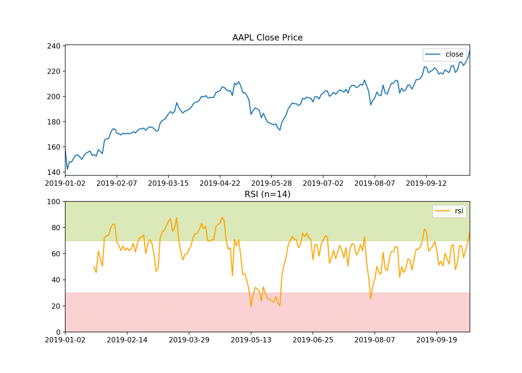
import matplotlib.gridspec as gridspecThen after computing the RSI we can create a window and show our plots. Since the RSI and our stock price use different axes we will use subplots to display both values on separate plots. We also add a bit of styling and fill the overbought and oversold regions of the RSI plot.
# set up plots and axes for plotting
fig = plt.figure()
gs = gridspec.GridSpec(2, 1)
ax1 = plt.subplot(gs[0, 0])
ax2 = plt.subplot(gs[1, 0])

# fill overbought and oversold regions on RSI plot
ax2.set_ylim([0, 100])
ax2.fill_between(stock.index, 70, 100, color='#a6c64c66')
ax2.fill_between(stock.index, 0, 30, color='#f58f9266')

# display xaxis labels nicely
ax2.set_xticks(stock.index[::30])
fig.add_subplot(ax1)
fig.add_subplot(ax2)

# plot our stock values
stock[['close']].plot(ax=ax1, title=f'{SYMBOL} Close Price')
stock[['rsi']].plot(ax=ax2, color='orange', title='RSI (n=14)')

# show the window
plt.show()
You’ll notice that we select each column before calling plot. Feel free to add values to this list to plot additional lines on the same plot. There we have it, with just a few lines of code we have a beautiful plot of stock price in matplotlib:
I highly recommend you take a look at the documentation for matplotlib as there are numerous options for displaying your plots.
Summary
In today’s blog post you have learned how to do simple stock analysis with Python. We’ve covered a variety of core stock analysis topics including:
- Downloading stock data with Pandas Data Reader library
- Performing technical analysis with Python
- Graphing stock data with matplotlib and Python
With an understanding of these core fundamentals you can begin developing your own quantitative trading strategies and systems.
Keep an eye out for my upcoming posts on stock analysis with Python. If you have any questions using the code discussed in this article, please don’t hesitate to reach out in the comments!